Mismatch

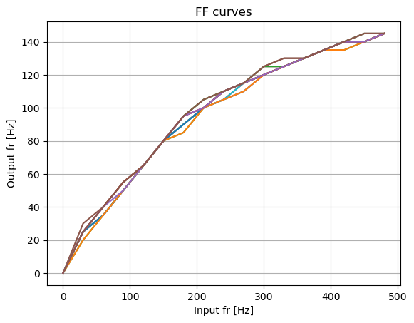
On this experiment we are going calculate the FF curve for different neurons with a mismatch of 10% on the synaptic weights. First, we are going to import the necesary libraries and set the simulation timestep.

import torch
import torch.nn as nn
import numpy as np
import matplotlib.pyplot as plt
from tqdm import trange

from DynapSEtorch.model import AdexLIF

timestep = 100 * 1e-6

Input generation

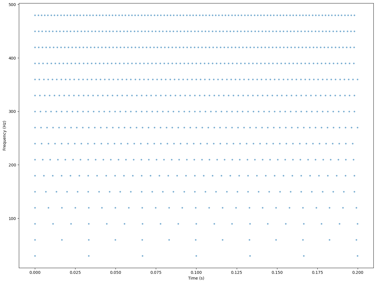
We are going to create a total of 16 neurons with an input spike frequency in the range [0, 500]Hz in steps of 30Hz

num_neurons = 16
freq = np.arange(0, 500, 30)

# Parameters
pulse_start = 0  # second - Start time of input (Default: 0)
pulse_stop = 1  # second - Stop time of input (Default: 5)
inp_duration = 0.2  # second - Simulation duration (Default: 5)
rate = 30  # Hz or rad/sec - Spiking rate (Default: 80 Hz for regular, 100 Hz for poission, 2 rad/sec for cosine)
##################

spikes = torch.zeros(len(freq), int(inp_duration / timestep))

for i, rate in enumerate(freq[1:]):
    dt = int((1 / timestep) / rate)
    spikes[
        i + 1, pulse_start * int(1 / timestep) : pulse_stop * int(1 / timestep) : dt
    ] = 1.0

input = spikes.unsqueeze(2).cuda()

b, t = np.where(spikes)
plt.figure(figsize=(16, 12))
plt.scatter(t * timestep, freq[b], marker=".", alpha=0.5)
# plt.yscale(u'log')
plt.ylabel("Frequency (Hz)")
plt.xlabel("Time (s)")

Text(0.5, 0, 'Time (s)')

Model creating and simulation

Once we created the input, we instantiate a layer of 16 AdexLIF neurons with an AMPA synapse connected to each input. The simulation is processed in batches, where each batch correspond to a determinated frequency.

network = AdexLIF(num_neurons=16, input_per_synapse=[0, 1, 0, 0]).cuda()
network.dt = timestep
output = []

with torch.no_grad():
    network.weight_ampa.data = torch.ones_like(network.weight_ampa.data) * 5
    network.state = network.init_state(input[:, 0])
    for t in trange(input.shape[1]):
        output.append(network(input_ampa=input[:, t]))
    output_mean = torch.stack(output, dim=1).detach().cpu()

100%|██████████| 2000/2000 [00:13<00:00, 146.35it/s]

plt.plot(freq, output_mean.sum(dim=1) / inp_duration)
plt.xlabel("Input fr [Hz]")
plt.ylabel("Output fr [Hz]")
plt.title("FF curves")
plt.grid()
plt.show()